ipypm - MCMC tab

The MCMC tab allows you to produce a projection of population sizes along with 95% confidence belts. The method for defining the posterior probably density for the MCMC process is described in the pypmca documentation here.

There are several steps required:

1. In the Explore tab, set n_days to show the projection period into the future. Hit “Plot” to see if that looks right.
2. In the Analyze tab, you need to have defined the variable parameters and done a fit, to define the reference model with which the MCMC analysis is based.
3. In the MCMC window, add any additional variables you wish to include and specify normal priors for them. If these variables affect the data used in the Analyze tab, they should have been set for that analysis and you should the analysis again with them included. In this example, the fraction of symptonatic people entering ICU is added as a variable, with the prior mean = 0.03 (the point estimate from the data fit) and its standard deviation set arbitrarily to 0.01, for illustration.
4. Set MCMC step sizes for each variable. In general the step sizes should be a fraction of their one-sigma uncertainty. If these are not known, use your best guess. After starting MCMC (see below) you will see the fraction of MCMC steps accepted. If that number is less than 0.3, you should reduce the MCMC step size. If that number is larger than 0.9, you should increase the step size… these are just rough guidelines!
5. Click on the show variables to see that all variables are ready. See image below.
6. Calculate the autocovariance (button)
7. Calculate the goodness of fit statistics for simulated samples (cal sim gof button). This will print the values as shown in the image below: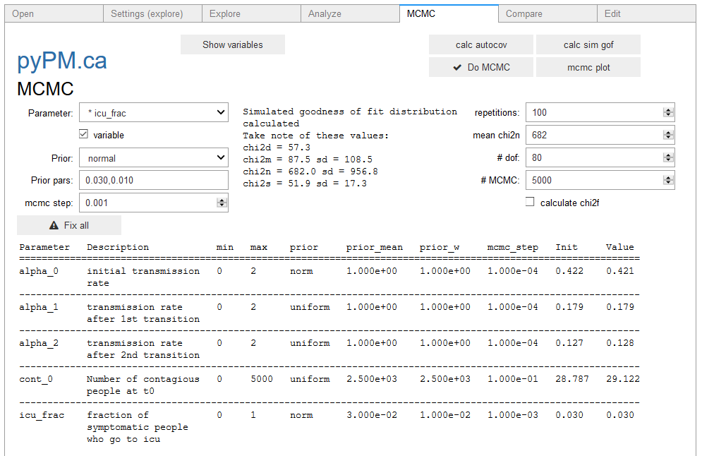
8. Enter the chi2_n number into the text box. This is used in the normalization part of the likelihood calculation.
9. Enter a number of degrees of freedom, which is used in the shape part of the likelihood calculation.
10. Choose the number of MCMC points to produce. 5000 will take a couple of minutes. Choosing more points means that more of the parameter space is explored.
11. Produce the chain of MCMC points (click the Do MCMC button). The chain is available for inspection: my_ipypm.chain An example is shown how to visualize the chain using pandas below.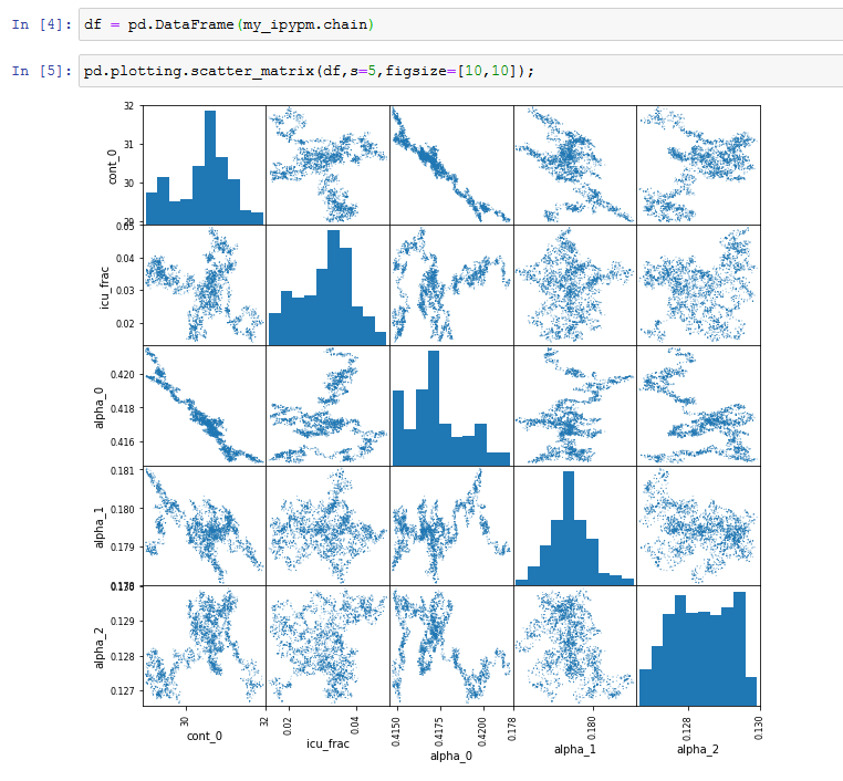
12. Produce the projection plot with 95% CL bands by clicking on the mcmc plot button. This plot is generated by selecting a random sample of the MCMC points, producing simulated data for those, and showing the central 95% of their deviations from the expectation.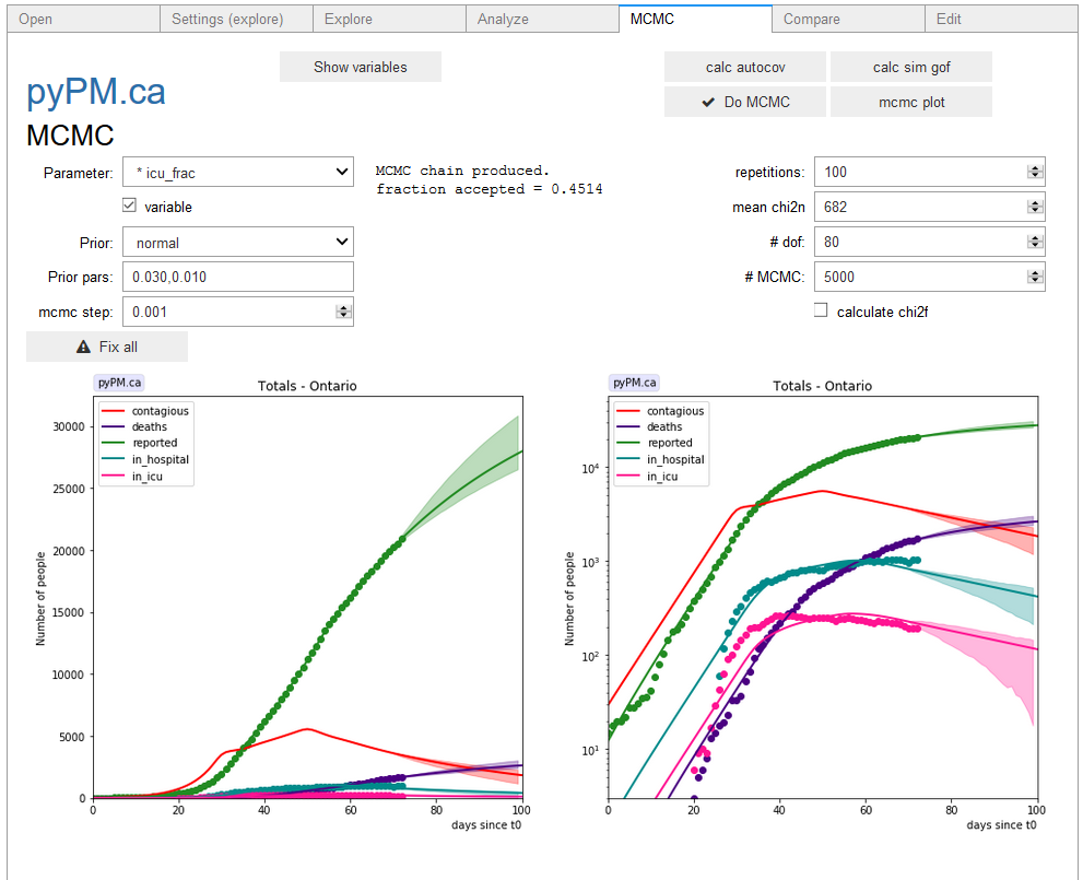

This example shows a projection for constant transmission rate. Alternatively, a projection with a transition to a new (uncertain) transmission rate can be considered, by adding the transition to the model and entering the prior belief for the future transmission rate.