December 6, 2020 Analysis of German state data
This shows the results of fits to data from the 16 German states. This updates the earlier study which described in detail as in the paper Charaterizing the spread of CoViD-19.
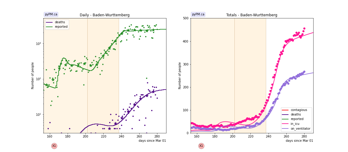
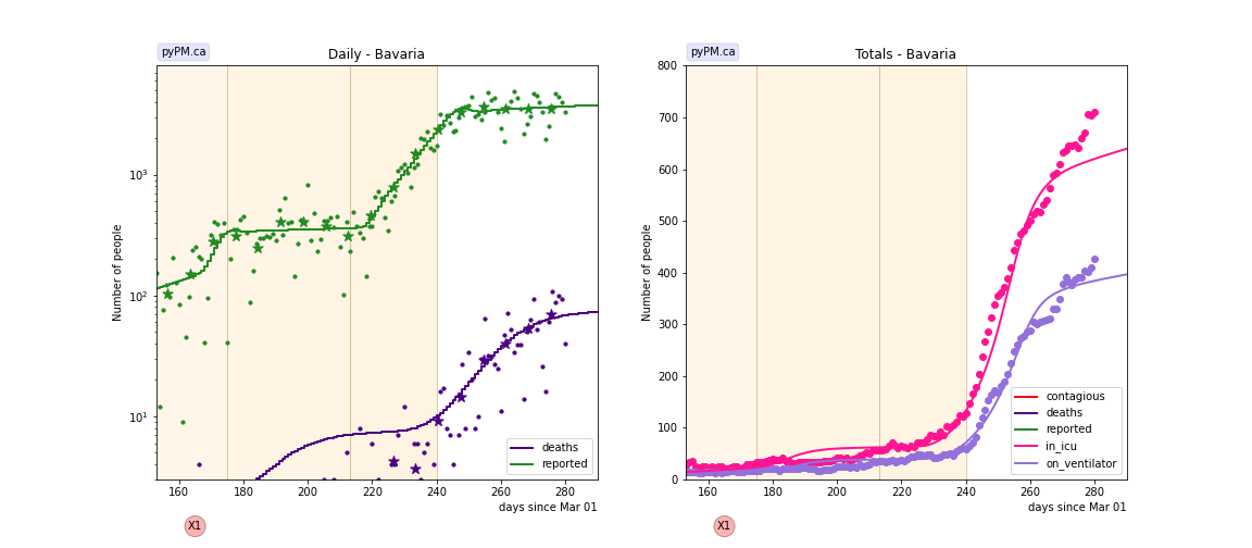
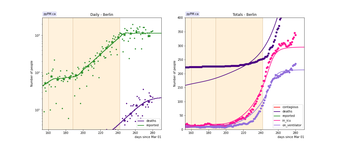
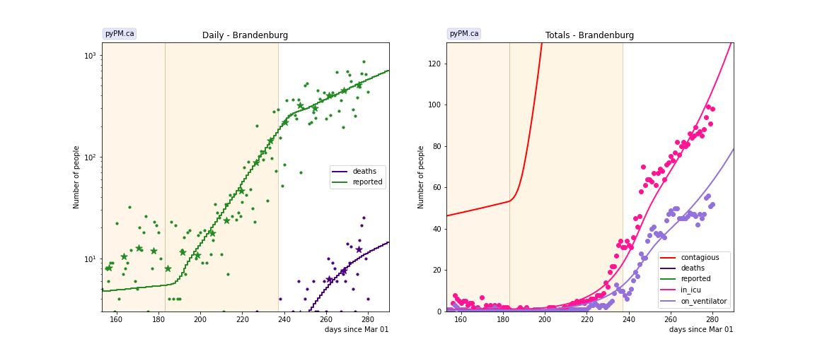
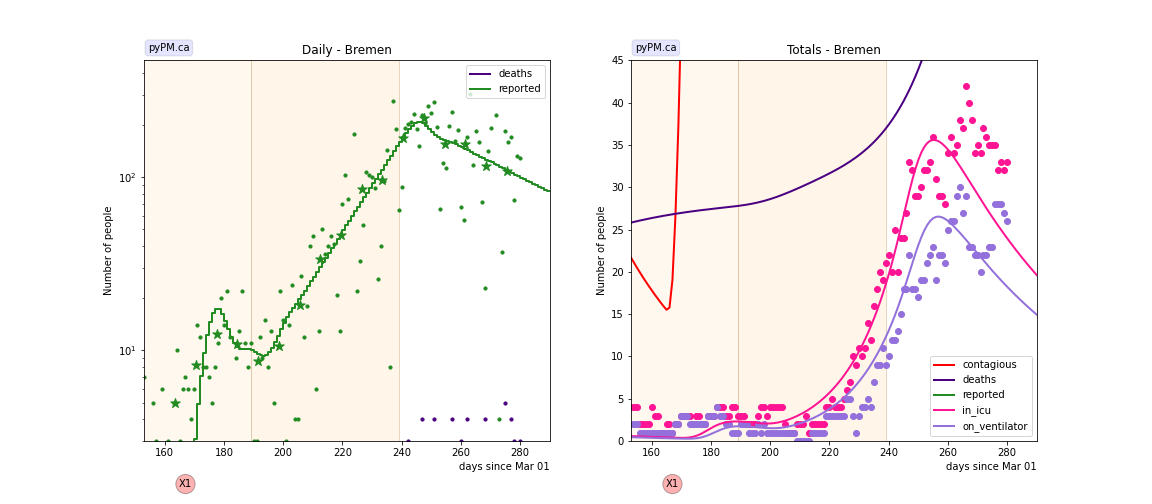
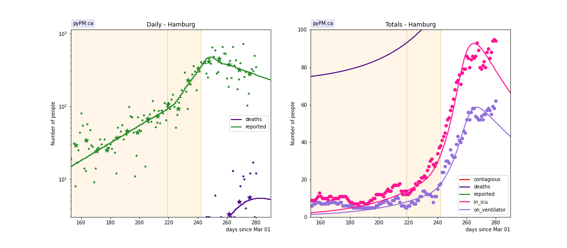
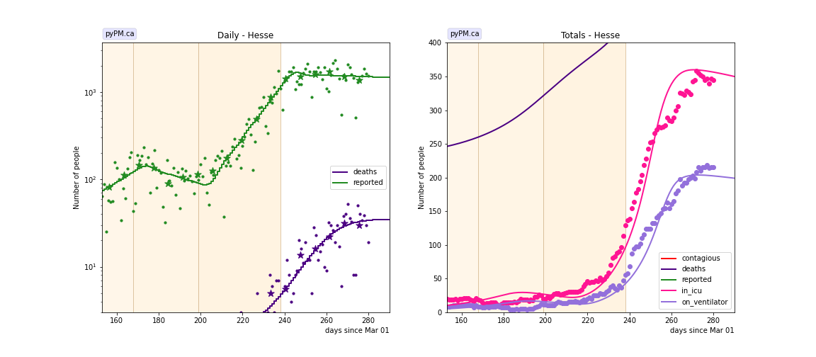
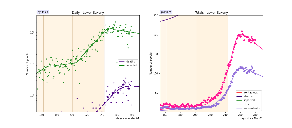
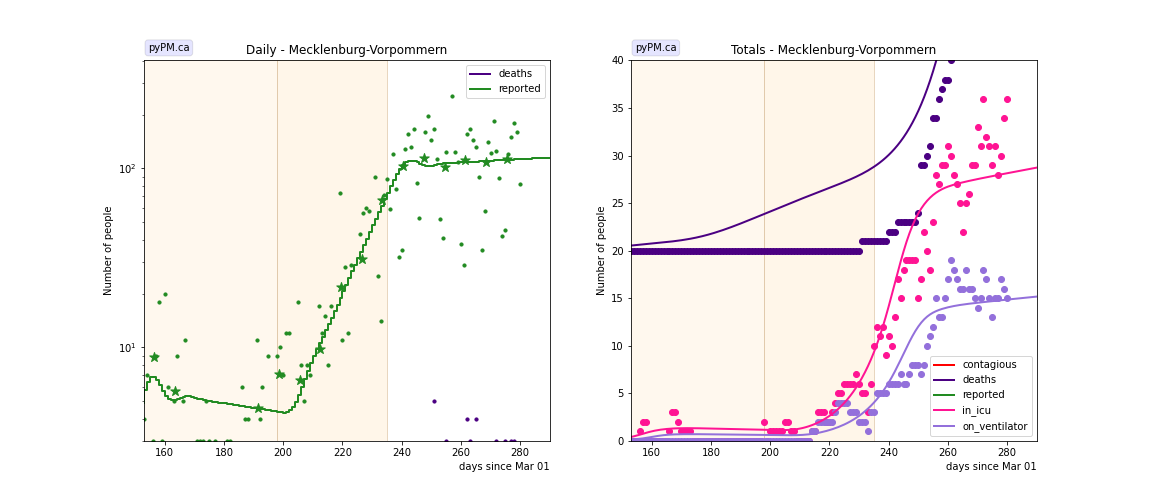
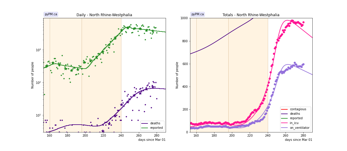
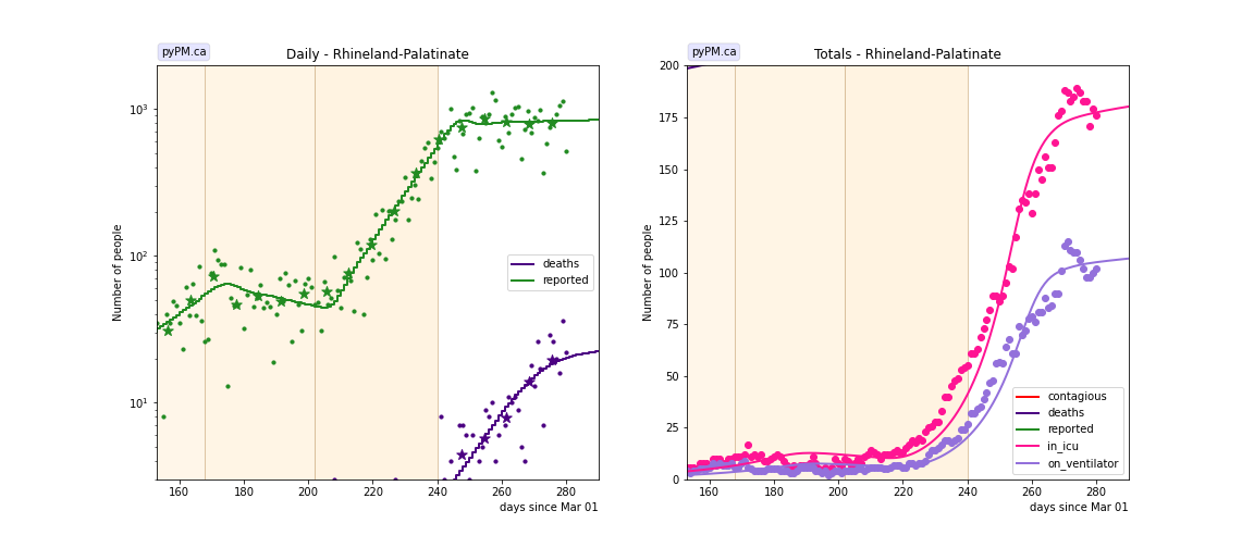
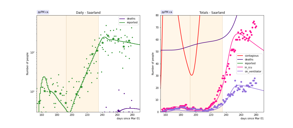
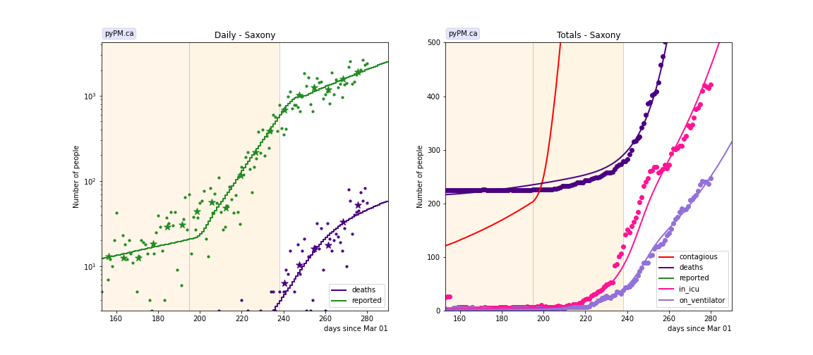
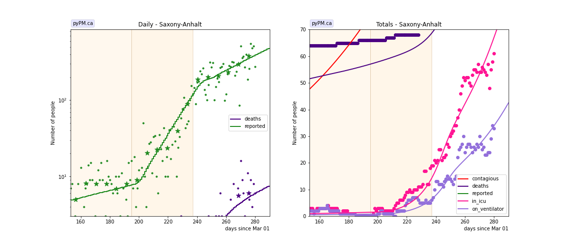
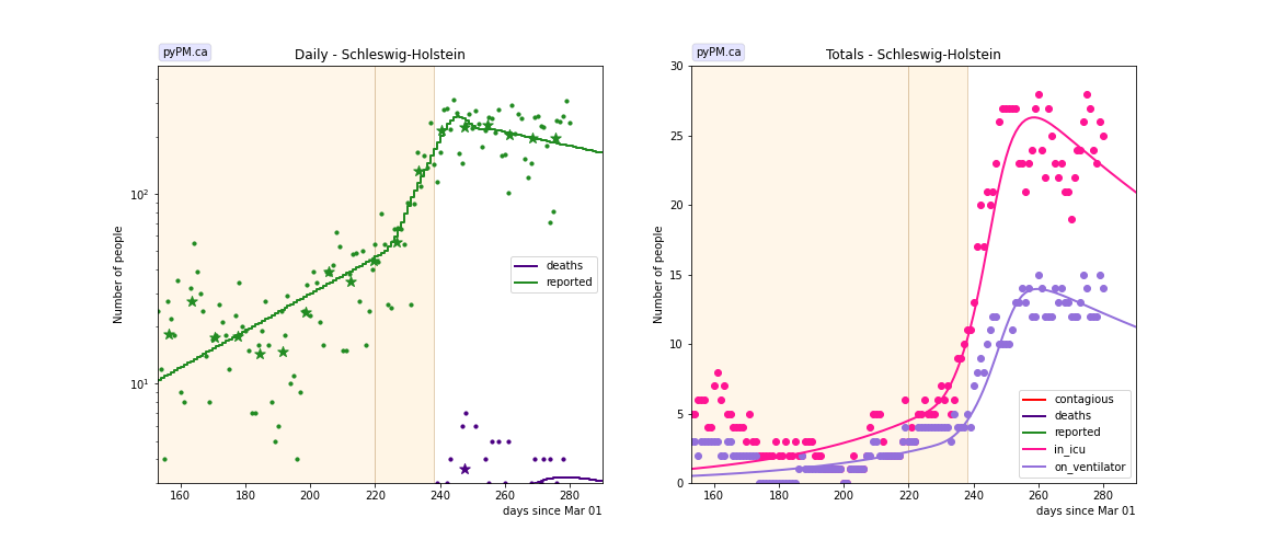
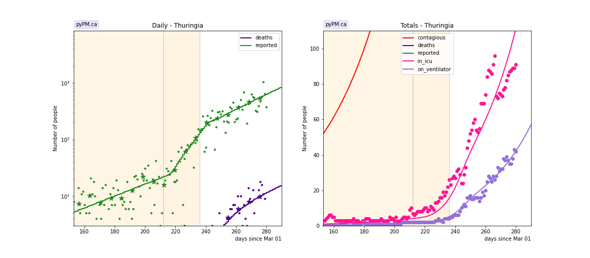
The left figures below, show the daily case history since August 1, 2020, on a log scale. The points daily data, and the stars show the weekly average and the pypm model is fit to this data to determine the infection trajectory. That trajectory is itself defined by long periods of constant transmission rates.
The curves show the model predictions given the transmission rate parameters, as determined from the case data only. The shaded regions indicate the periods having a constant transmission rate.
The model parameter for the mean time from infectiousness to death needed to be increased from 18 days, as found in the April data, to around 30 days for the recent data.
The right figures show the number of patients in ICU and on ventilators.
Studies broken down by age are shown below.
Baden-Wurttemberg
Bavaria
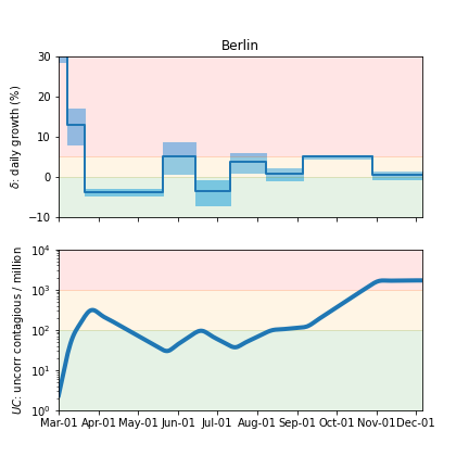
Berlin
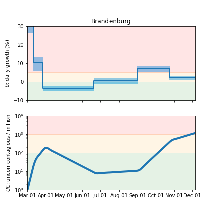
Brandenburg
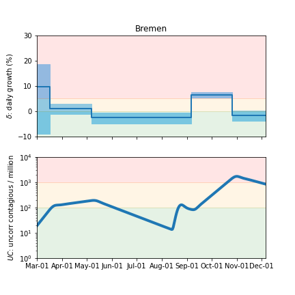
Bremen
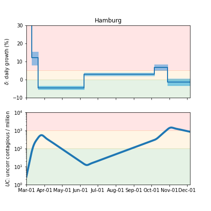
Hamburg
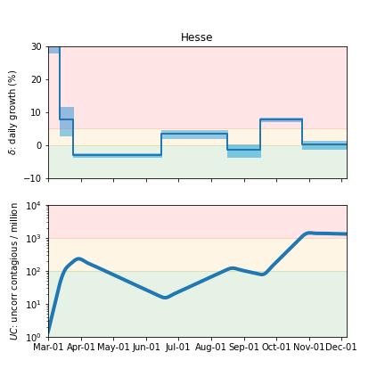
Hesse
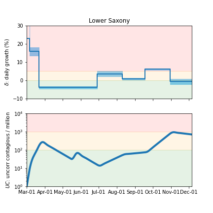
Lower Saxony
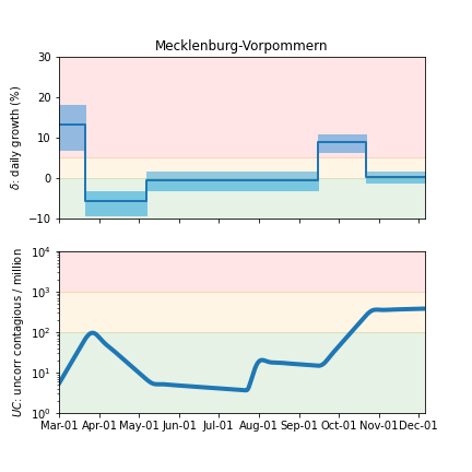
Mecklenburg-Vorpommern
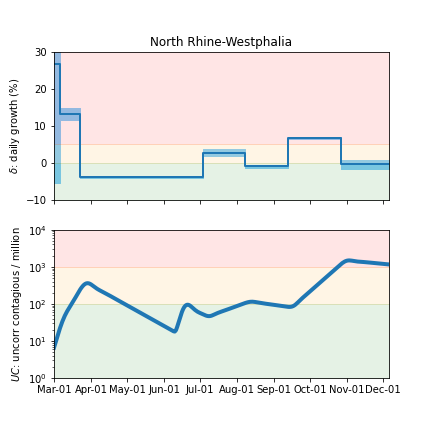
North Rhine-Westphalia
Rhineland-Palatinate
Saarland
Saxony
Saxony-Anhalt
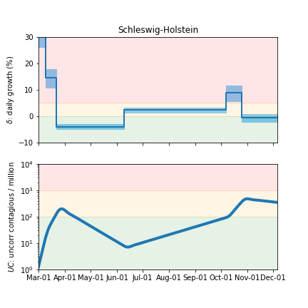
Schleswig-Holstein
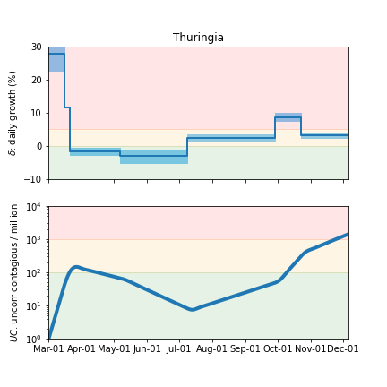
Thuringia
Tables
daily growth/decline rates (δ)
Shown are growth rates (% per day) since August 1, with the date of the transition. 68% confidence intervals shown.
| state | δ | day | δ | day | δ | day | δ |
|---|---|---|---|---|---|---|---|
| BW | -1.8 +/- 0.3 | Sep 19 | 7.6 +/- 0.2 | Oct 24 | 0.6 +/- 0.5 | ||
| BY | 2.4 +/- 0.9 | Aug 23 | 0.4 +/- 0.4 | Sep 30 | 8.4 +/- 0.3 | Oct 27 | 0.7 +/- 0.5 |
| BE | 3.8 +/- 1.2 | Aug 08 | 0.8 +/- 0.8 | Sep 05 | 5.1 +/- 0.2 | Oct 29 | 0.4 +/- 0.5 |
| BB | 0.6 +/- 0.8 | Aug 31 | 7.2 +/- 0.7 | Oct 24 | 2.4 +/- 0.5 | ||
| HB | -2.5 +/- 1.1 | Sep 06 | 6.5 +/- 0.5 | Oct 26 | -1.6 +/- 1.1 | ||
| HH | 2.9 +/- 0.4 | Oct 06 | 6.8 +/- 0.9 | Oct 29 | -1.2 +/- 1.0 | ||
| HE | 3.5 +/- 0.6 | Aug 16 | -1.5 +/- 0.9 | Sep 16 | 7.8 +/- 0.3 | Oct 25 | 0.2 +/- 0.6 |
| NI | 3.6 +/- 0.8 | Aug 10 | 0.8 +/- 0.3 | Sep 18 | 6.2 +/- 0.2 | Oct 30 | -0.6 +/- 0.8 |
| MV | -0.5 +/- 1.2 | Sep 15 | 8.8 +/- 1.1 | Oct 22 | 0.4 +/- 0.7 | ||
| NW | 2.8 +/- 0.4 | Aug 08 | -0.8 +/- 0.2 | Sep 13 | 6.9 +/- 0.1 | Oct 27 | -0.3 +/- 0.7 |
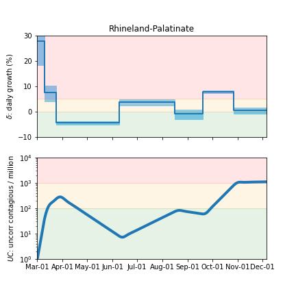
| RP | 3.8 +/- 0.6 | Aug 16 | -0.9 +/- 1.0 | Sep 19 | 7.8 +/- 0.3 | Oct 27 | 0.4 +/- 0.6 |
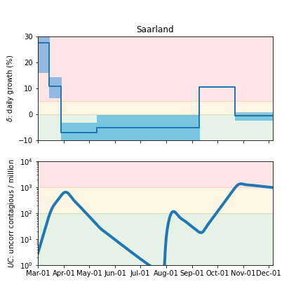
| SL | -5.1 +/- 3.2 | Sep 09 | 10.7 +/- 8.4 | Oct 22 | -0.5 +/- 0.8 | ||
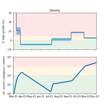
| SN | 1.3 +/- 0.8 | Sep 12 | 8.8 +/- 0.4 | Oct 25 | 2.6 +/- 0.4 | ||
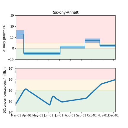
| ST | 1.2 +/- 0.6 | Sep 12 | 7.3 +/- 0.9 | Oct 24 | 2.5 +/- 0.5 | ||
| SH | 2.3 +/- 0.4 | Oct 07 | 8.9 +/- 1.5 | Oct 25 | -0.6 +/- 0.7 | ||
| TH | 2.5 +/- 0.6 | Sep 29 | 8.8 +/- 0.6 | Oct 23 | 3.3 +/- 0.4 |
hospitalization and death parameters
Some model parameters can be estimated with these data. 68% CL intervals are shown.
| state | rec. frac | death delay | icu frac | icu delay | vent_frac | vent delay |
|---|---|---|---|---|---|---|
| BW | 0.984 +/- 0.002 | 35.4 +/- 3.7 | 0.011 +/- 0.002 | 8.4 +/- 2.1 | 0.82 | 3.5 +/- 1.1 |
| BY | 0.985 +/- 0.002 | 30.7 +/- 5.8 | 0.011 +/- 0.003 | 10.6 +/- 0.9 | 0.83 | 3.2 +/- 1.8 |
| BE | 0.986 +/- 0.004 | 35.7 +/- 7.4 | 0.016 +/- 0.006 | 4.6 +/- 2.8 | 0.95 | 3.1 +/- 3.1 |
| BB | 0.972 +/- 0.007 | - | 0.014 +/- 0.006 | - | 0.81 | - |
| HB | 0.989 +/- 0.003 | - | 0.012 +/- 0.005 | - | 0.96 | - |
| HH | 0.990 +/- 0.003 | - | 0.013 +/- 0.005 | 9.6 +/- 2.5 | 0.89 | 4.3 +/- 1.3 |
| HE | 0.984 +/- 0.004 | 31.5 +/- 3.9 | 0.012 +/- 0.006 | 9.4 +/- 1.3 | 0.86 | 5.3 +/- 2.3 |
| NI | 0.988 +/- 0.002 | 27.4 +/- 5.8 | 0.011 +/- 0.004 | 4.4 +/- 2.0 | 0.68 | 1.2 +/- 0.8 |
| MV | 0.982 +/- 0.003 | - | 0.015 +/- 0.005 | - | 0.74 | - |
| NW | 0.989 +/- 0.001 | 26.8 +/- 3.2 | 0.014 +/- 0.002 | 6.2 +/- 0.5 | 0.78 | 2.6 +/- 0.9 |
| RP | 0.979 +/- 0.005 | 36.5 +/- 5.9 | 0.012 +/- 0.004 | 10.7 +/- 2.0 | 0.83 | - |
| SL | 0.987 +/- 0.003 | - | 0.017 +/- 0.004 | - | 0.48 | - |
| SN | 0.971 +/- 0.007 | - | 0.016 +/- 0.006 | - | 0.81 | - |
| ST | 0.981 +/- 0.006 | - | 0.012 +/- 0.004 | 3.7 | 0.67 | - |
| SH | 0.989 +/- 0.002 | - | 0.007 +/- 0.003 | - | 0.74 | - |
| TH | 0.973 +/- 0.006 | - | 0.013 +/- 0.005 | - | 0.57 | - |
- rec. frac: fraction of contagious who recover (for relative comparison only)
- death delay: mean number of dates from infectious to death
- icu frac: fraction of symptomatic who are admitted to ICU
- icu delay: mean time from symptoms to ICU admission
- vent frac: fraction of icu patients who are intubated
- vent delay: mean time from ICU admission to ventilator
Notes:
-
The following parameter values were assumed:
- Mean time in ICU: 14 days
- Mean time on ventillator: 10 days
-
Changing these parameter values would affect the estimates for icu frac, since the current number of patients in the ICU depends on the length of time patients stay in the ICU.
-
Also, the fraction of the infected population that were tested is not well established, which means that the absolute fraction of contagious who die is not well known. The rec. frac is therefore useful only for relative comparison only.
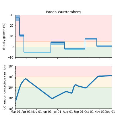
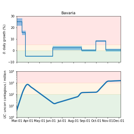
Infection status
The following plots summarize the infection history. The upper plot shows the daily growth/decline from the fit. Bands show approximate 95% CL intervals. The lower plot shows the size of the infection: the uncorrected circulating contagious population per million.
Baden-Warttemberg
Bavaria
Berlin
Brandenburg
Bremen
Hamburg
Hesse
Lower Saxony
Mecklenburg-Vorpommern
North Rhine-Westphalia
Rhineland-Palatinate
Saarland
Saxony
Saxony-Anhalt
Schleswig-Holstein
Thuringia
Studies by age
Different age groups generally do not follow the social distancing policies to the same extent. Despite that, the epidemic growth is typically very similar between the groups, and this can be explained by mixing between the groups.
The most recent change to transmission rates occuring at the end of October shows an unusual trend with the older age groups having daily growth larger than the younger groups. An example is seen in the figure below that shows cases over the past 60 days in NW state, as fit with an ensemble of 4 age groups: (a2: 15-34, a3: 35-59, a4:60-79, a5:80+).
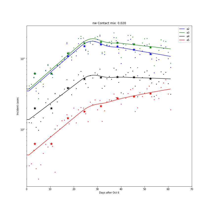
This may be the reason that the ICU and ventilator data do not follow the homogeneous model predictions over the past few weeks in some states, as shown above. ICU and ventilator data by age group is not available.
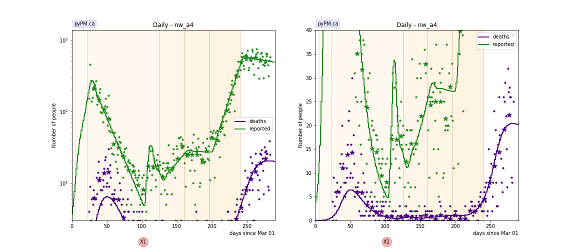
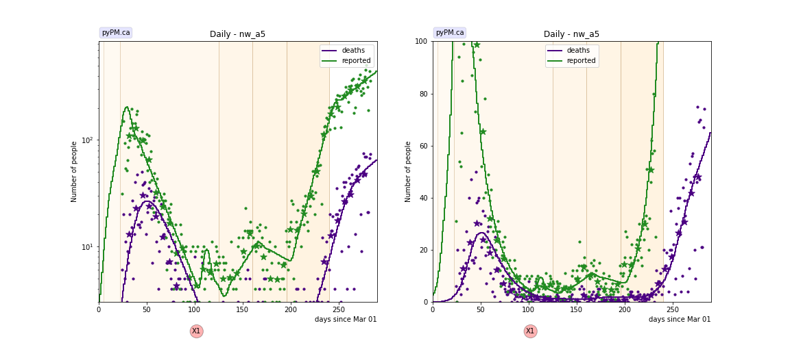
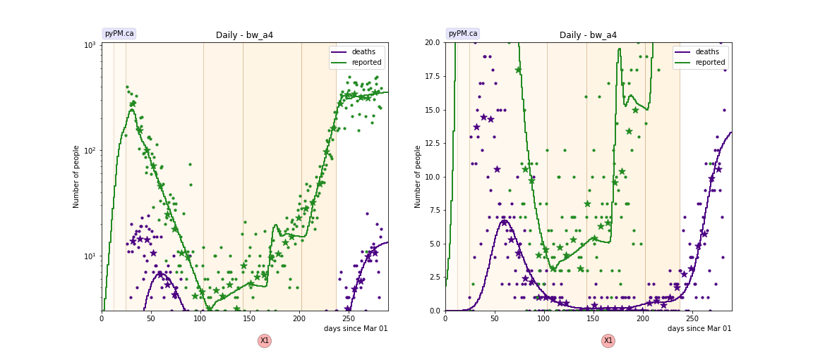
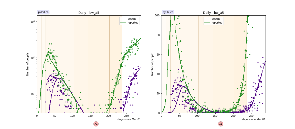
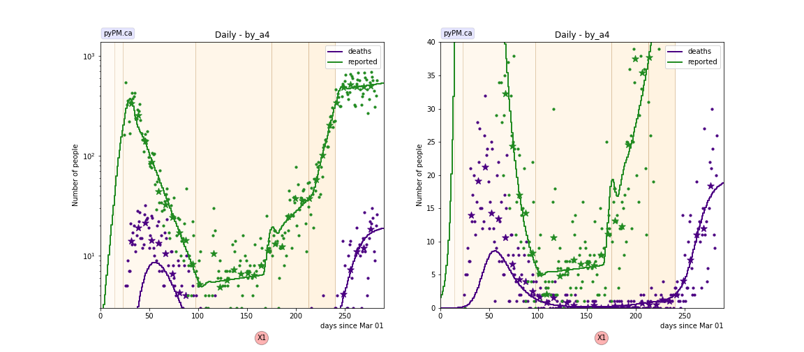
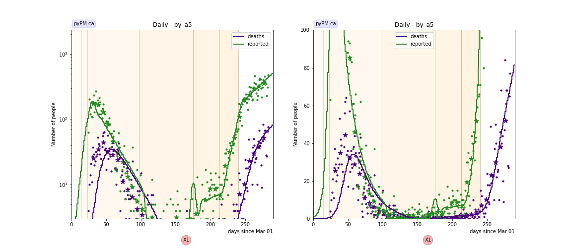
Cases and deaths by age
The following figures shows cases and deaths in the older age groups for three states, Baden-Warttemberg (bw), Bavaria (by), and North Rhine-Westphalia (nw), where the labels are (a4: age 60-79, a5: age 80+).
The main features (transition dates, dates of outbreaks) are taken from the homogenous fits for each state. Also, the death delays assumed in the fits are those estimated from the homogeneous model fits above. The transmission rates and scaling parameters are adjusted for each age group.
[Baden-Warttemberg]
[Bavaria]
[North Rhine-Westphalia]