June 17, 2020 Analysis of German state data (with updates on June 20)

Data from March 1-June 10 were included in the June 17 analysis. Strick lockdown in Germany started on March 22. The transition date for the transmission rates were not fixed to that date: most fits found the transition to be very close to March 22.

Relaxation of lockdown rules started on May 6. To evaluate the effect on the spread of CoViD-19, a transition is transmission rate was imposed on that date, and the transmission rates before and after were fit.

The results from the 16 German states are remarkably consistent with similar values for δ before and after the imposition of the lockdown rules. There is no significant increase in δ after the relaxation.

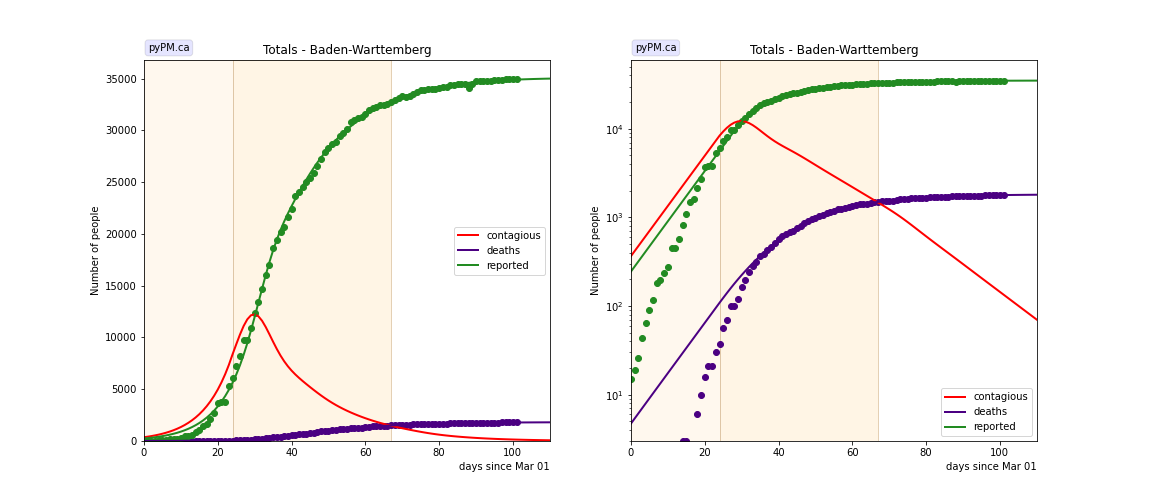
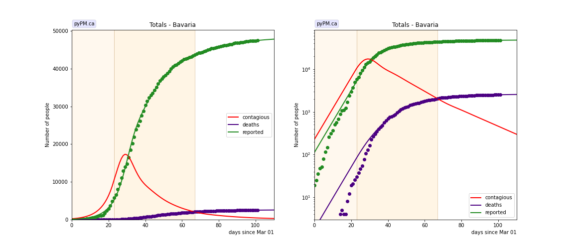
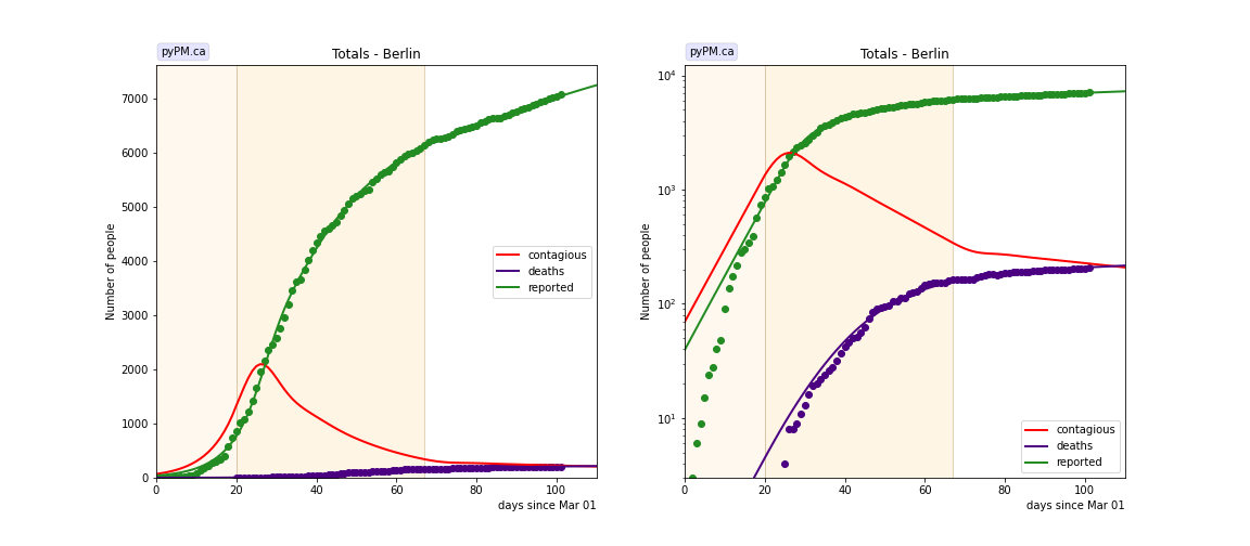
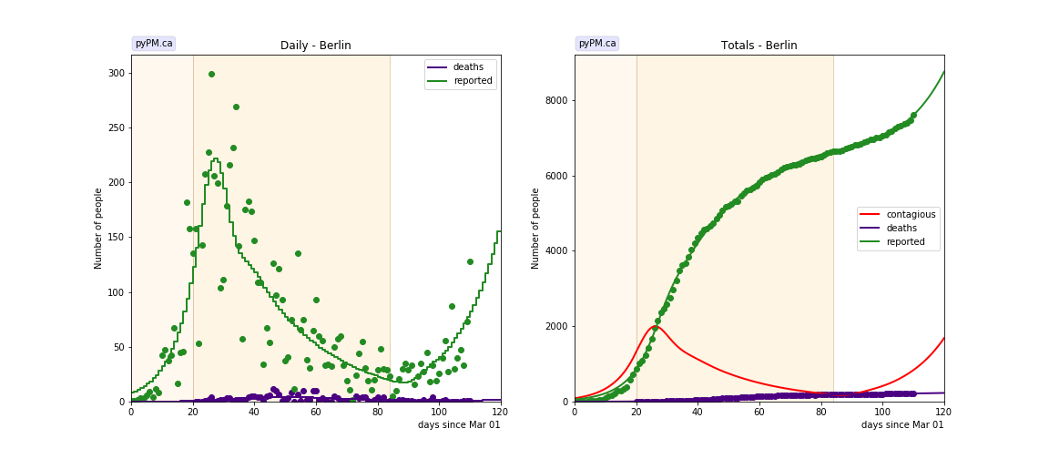
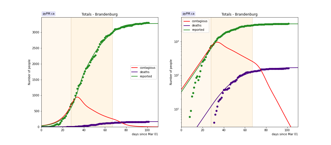
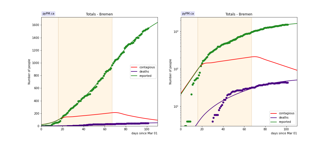
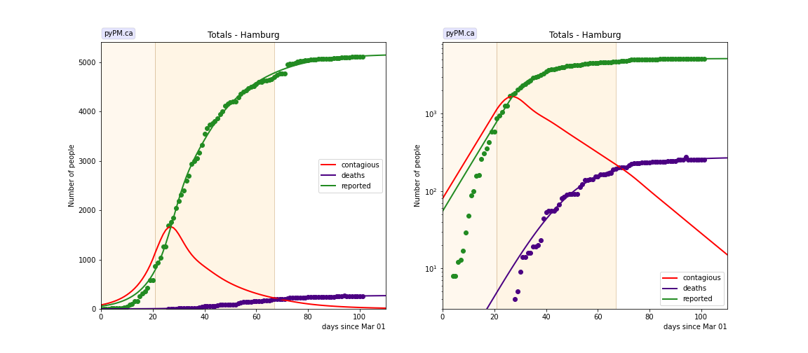
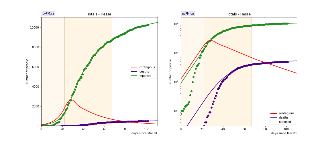
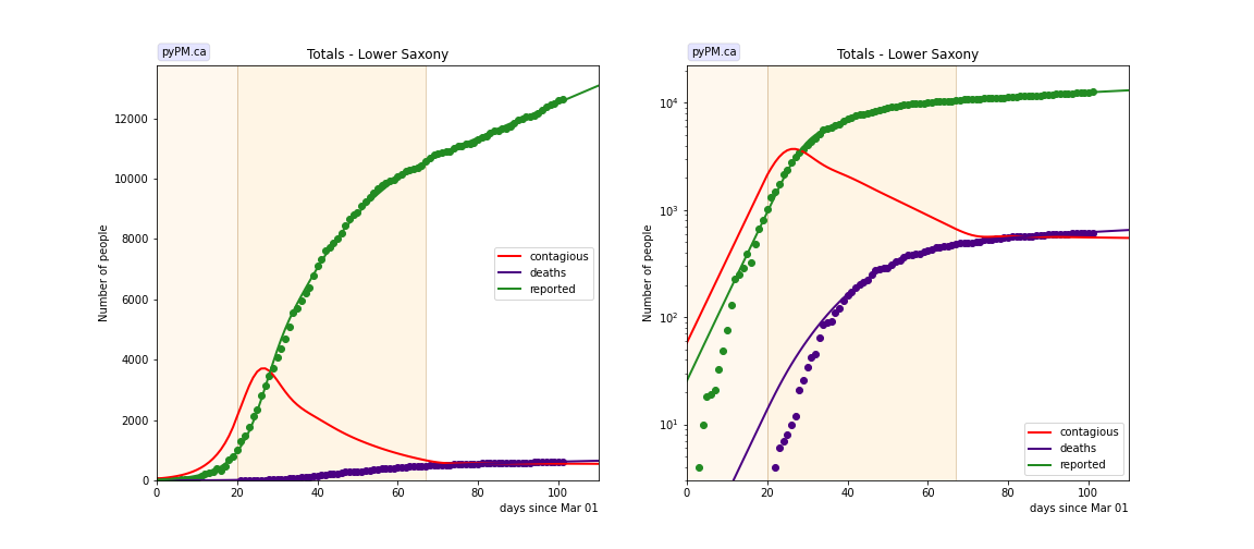
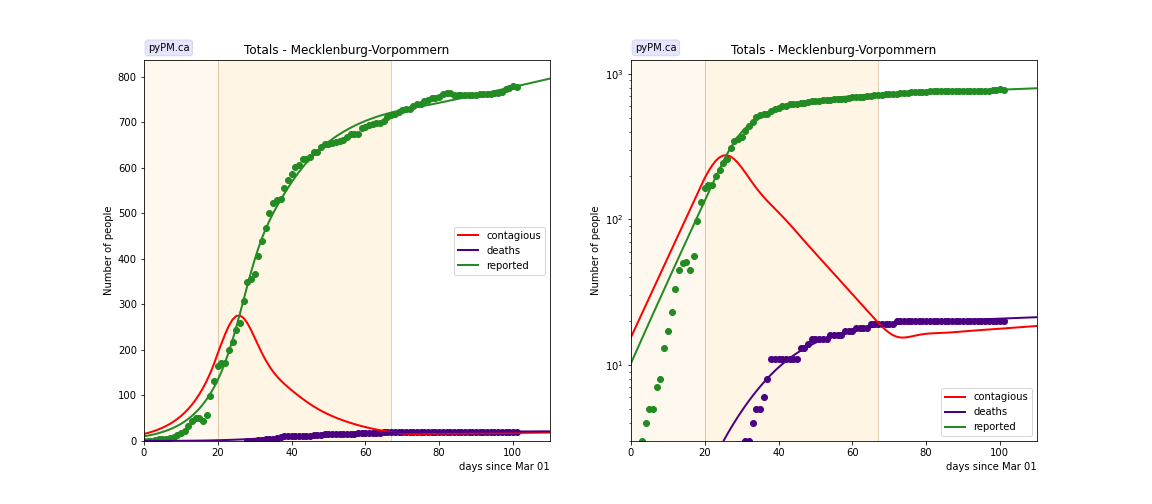
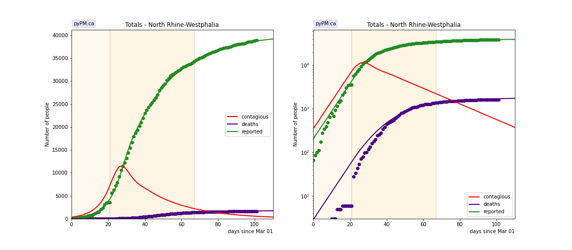
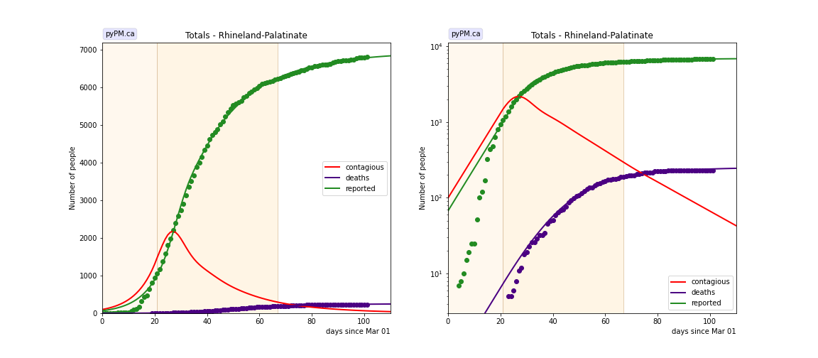
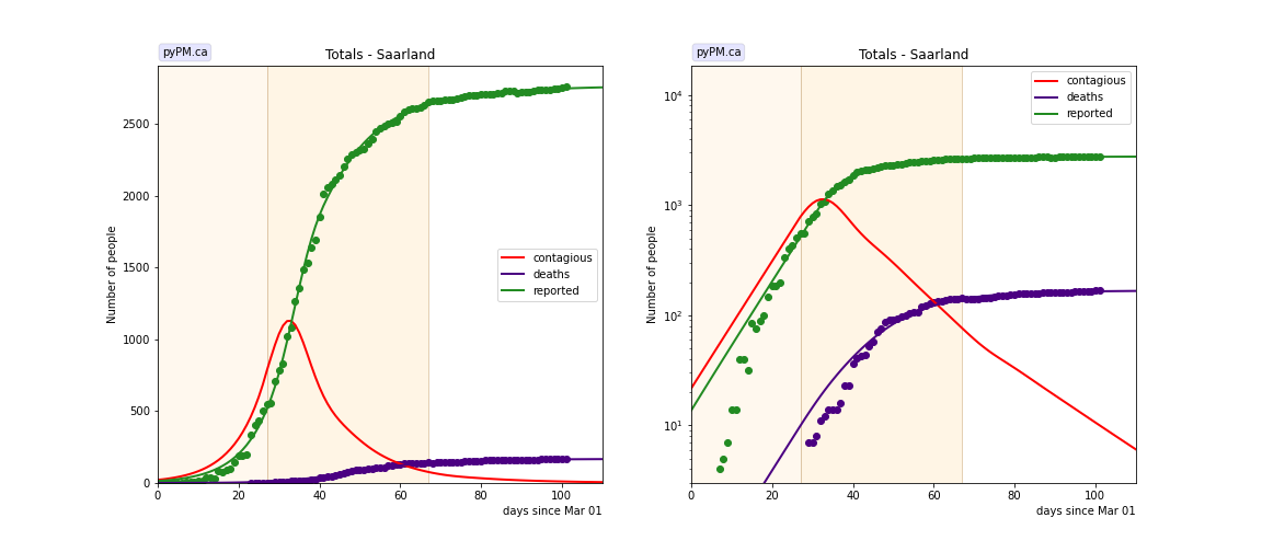
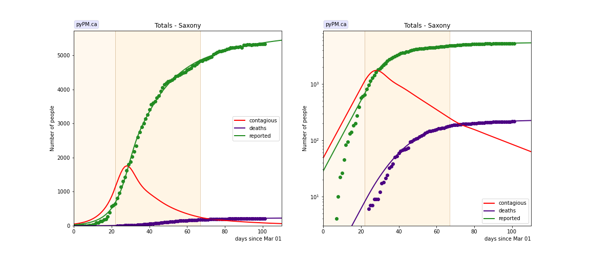
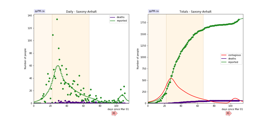
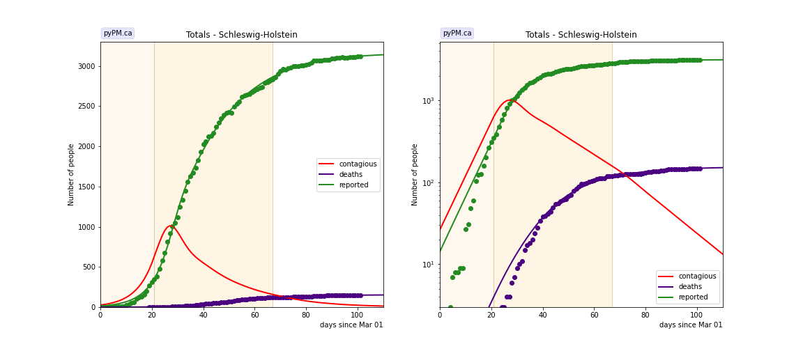
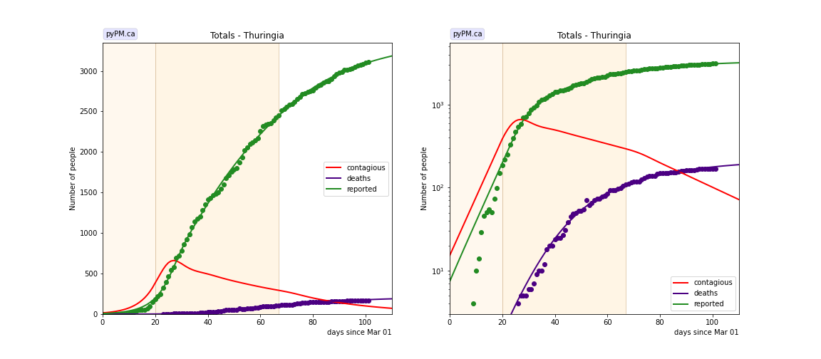
Below shows the case and deaths data for all 16 states compares to the pypm model fit to the case data.

The red curves (contagious population) is the inferred contagious population. Its shape is determined from the case data. Its scale is not well known.

Following are tables and figures comparing the different states as well as the infection status plots, that summarize the growth and size of the epidemic. PDF versions of plots are available by clicking on the titles

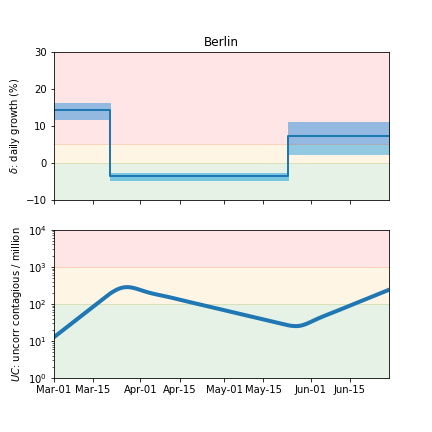
Update June 20: By including data through June 19, it now appears that Berlin is experiencing exponential growth, transition date: May 23. The state of Saxony-Anhalt has also recently seen a rapid rise in new cases. It is possible that these recent rises in cases are due to localized outbreaks. Revised versions are shown below.

Baden-Warttemberg

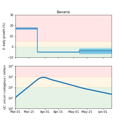
Bavaria

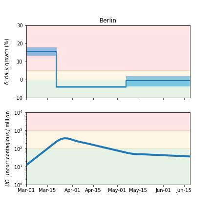
Berlin through June 10

Berlin through June 19

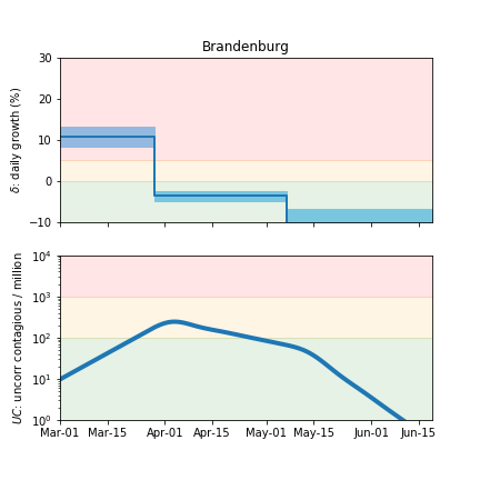
Brandenburg

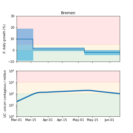
Bremen

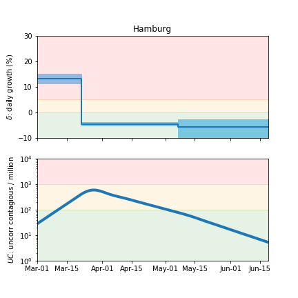
Hamburg

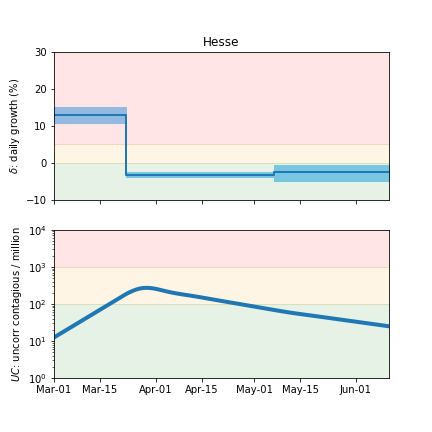
Hesse

Lower Saxony

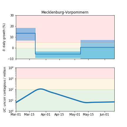
Mecklenburg-Vorpommern

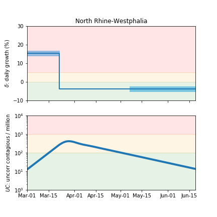
North Rhine-Westphalia

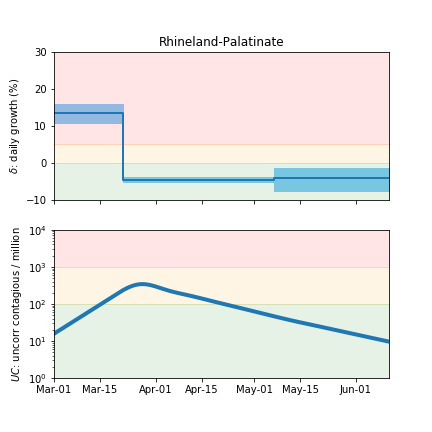
Rhineland-Palatinate

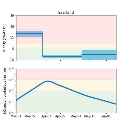
Saarland

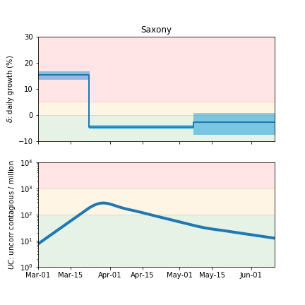
Saxony

Saxony-Anhalt through June 10

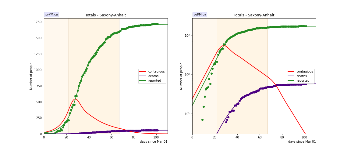
Saxony-Anhalt through June 20

Schleswig-Holstein

Thuringia

Tables

The tables below are results from the fits to reference model 2.3. These are shown for purposes of comparison.

daily growth/decline rates (δ)

state	δ₀	trans	δ₁	δ₂	f_d	d_d
bw	0.138 +/- 0.004	24	-0.050 +/- 0.001	-0.063 +/- 0.008	0.037	17.7
by	0.180 +/- 0.006	23	-0.049 +/- 0.002	-0.038 +/- 0.012	0.039	18.8
be	0.158 +/- 0.011	20	-0.039 +/- 0.002	-0.006 +/- 0.014	0.023	23.0
be*	0.142 +/- 0.011	20	-0.036 +/- 0.005	0.073 +/- 0.022	0.023	23.0
bb	0.109 +/- 0.012	28	-0.035 +/- 0.006	-0.118 +/- 0.045	0.037	18.4
hh	0.134 +/- 0.010	21	-0.044 +/- 0.003	-0.056 +/- 0.018	0.038	28.0
he	0.130 +/- 0.011	22	-0.031 +/- 0.004	-0.024 +/- 0.011	0.038	19.5
ni	0.195 +/- 0.014	20	-0.037 +/- 0.002	0.001 +/- 0.008	0.038	19.2
nw	0.155 +/- 0.007	21	-0.036 +/- 0.001	-0.036 +/- 0.007	0.033	18.9
rp	0.136 +/- 0.013	21	-0.044 +/- 0.004	-0.039 +/- 0.016	0.026	23.4
sl	0.141 +/- 0.014	27	-0.069 +/- 0.007	-0.050 +/- 0.025	0.044	19.0
sn	0.153 +/- 0.008	22	-0.044 +/- 0.004	-0.026 +/- 0.019	0.031	19.8
st	0.133 +/- 0.020	22	-0.042 +/- 0.010	-0.095 +/- 0.059	0.024	18.4
sh	0.162 +/- 0.027	21	-0.041 +/- 0.009	-0.052 +/- 0.032	0.035	21.0
th	0.174 +/- 0.028	20	-0.016 +/- 0.010	-0.030 +/- 0.019	0.046	24.4

be*: Berlin results through June 19
δ₀: initial δ, prior to lockdown
- mean value= 0.150, RMS= 0.022, mean stat error= 0.013
trans: fitted day of lockdown transition (actual date: 22)
- mean value= 22.3, RMS= 2.4
δ₁: δ after lockdown
- mean value= -0.041, RMS= 0.011, mean stat error= 0.005
δ₂: δ after relaxation on May 22
- mean value= -0.045, RMS= 0.031, mean stat error= 0.021
f_d: fatality rate
- mean value= 0.035, RMS= 0.007
d_d: mean time from contagious to death
- mean value= 20.7, RMS= 2.8

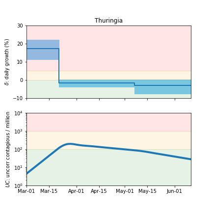
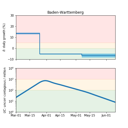
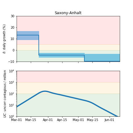
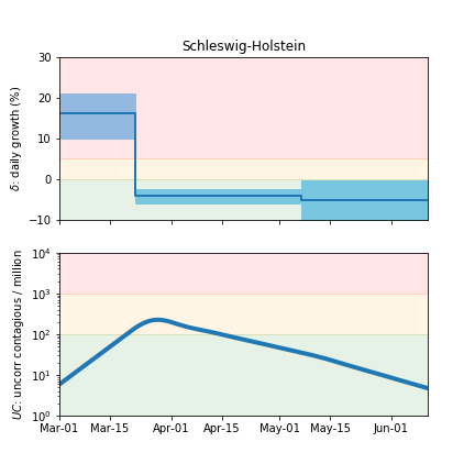
Infection status

The following plots summarize the infection history. The upper plot shows the daily growth/decline from the fit. Bands show approximate 95% CL intervals. The lower plot shows the size of the infection: the uncorrected circulating contagious population per million.